Computational Fluid Dynamics (CFD) encompasses a range of numerical methods and equations that allows simulation of fluid flows. This can provide engineers and scientists with the ability to test the impact of extreme conditions, model proposed changes, or see deep inside an operating plant without the need to build costly wind tunnel models or interrupt and tamper with an existing facility. Depending on the flow being simulated, a model with an appropriate complexity level can be adopted.
The first step in setting up a CFD simulation is to gain an understanding of the physics of the problem. This involves examining the problem in detail, and performing a few quick “back of the envelope” type calculations. Key questions to ask at this stage include:
- What is the geometry?
- Can the geometry be simplified to two dimensions? Although not always appropriate, when applicable, it can significantly reduce the computational cost, resulting in a faster turnaround time.
- Is the situation inherently steady or unsteady? For unsteady cases the solution fluctuates or changes as a function of time. Most flows are unsteady to at least a small level, but a steady solver can produce a time averaged solution that may produces adequate results. Steady solutions are preferable as they are much quicker to produce, unless unsteady effects are absolutely necessary.
- What are the inputs to this geometry? Does the system have a single phase input, or multiple phases? Multiple phase problems most commonly consist of air and either fuel and/or water but it could be any two fluids, or even a mixture of fluids and particulate solids like sand.
- Should the model include combustion? If so, what are the relevant chemical equations, and what level of details are needed for this combustion? One-step equations may suffice for some processes, while carbon monoxide and other by-products resulting from incomplete combustion may be a critical factor for others, necessitating the use of more detailed equations.
- Is heat flow and/or production relevant to the problem? If so, are there any heat inputs or losses that require modelling? Is the heat transferred by conduction, convection or radiation?
- Is the flow going to experience compression or shocks within the geometry? If the flow speeds exceed approximately 30% of the speed of sound, then the model should include compression effects as they may be significant. See Anderson [1] for details on why compressibility impacts only become relevant at high speeds.
- Will the flow be laminar or turbulent? Slow speed flows over smooth domains tend to be laminar, but most flows in engineering problems are turbulent.
Sometimes not all of the above questions will have a clear answer at first. In such cases, conducting background research or performing a sensitivity study becomes necessary. One can use sensitivity studies to assess a wide range of effects on a system solution. For instance, sensitivity studies can determine if the solution is unsteady or extract flow speeds from an initial, coarse simulation run to assess if compressibility is a concern before proceeding further.
Once the CFD engineer understands the physics behind the problem, they can build a computational model of the situation. This begins with a geometry model and construction of a computational mesh of cells in the region of fluid flow. These cells are used to provide a series of discrete locations where the governing fluid flow equations are solved. An adequately resolved mesh is critical for an accurate solution. Too coarse a mesh and the results from the subsequent simulation will be inaccurate, but too fine a mesh will produce an accurate solution, however the computations will take excessively long to calculate.
The image below displays an example of a finished mesh for solving the flow around a set of cylinders. It’s worth noting the fine resolution used between the two cylinders, in the immediate vicinity, and in the region where the wake is expected to occur.
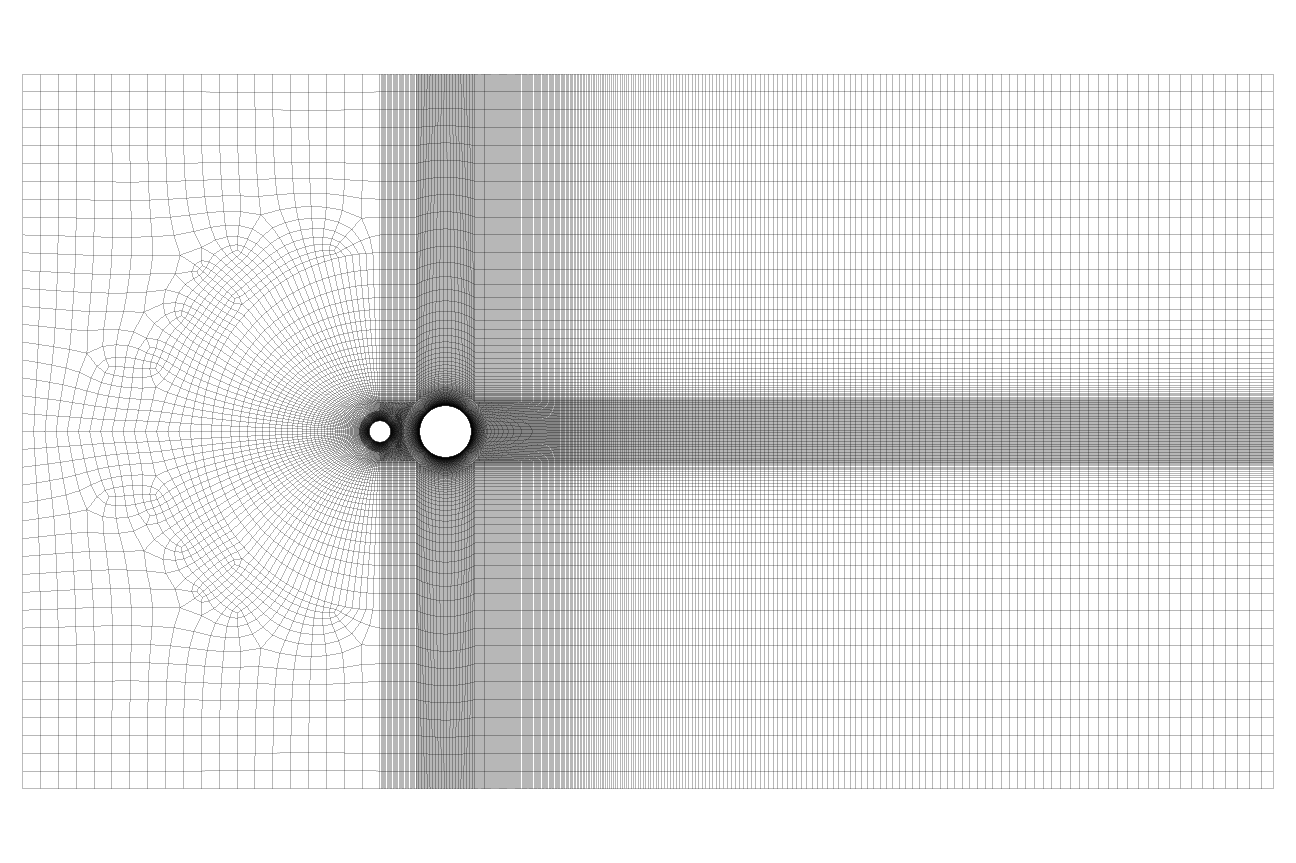
Figure 1: A 2D mesh around a pair of cylinders. We optimized the mesh to resolve a flow that travels from left to right.
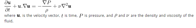
Next, one selects the appropriate numerical models and sets inputs based on the problem’s physics. The numerical models must efficiently and accurately solve each relevant component of the physics. The physics of the flow field is described by the Navier-Stokes equation,
Accurate, direct solution of the Navier-Stokes equation requires a very mesh to resolve the smallest eddies within the flow. For most situations this requires an impossibly high amount of computer power, in fact Spalart [2] estimates that solving these equations directly for a large aircraft, using a super computer will be feasible in approximately 2080! In the meantime, a Direct Numerical Simulation (DNS) of the Navier-Stokes Equations is only practical over small, simple geometries with low speed flows.
Instead, we use additional turbulence models to represent the behaviour of the smallest eddies without the need to directly model them, and save the computer power for modelling the larger scales. There a wide range of turbulence models in the CFD literature, each optimised in different ways. Depending on the physics of the problem a CFD engineer will select the most appropriate turbulence model. Turbulence modelling is an entire topic in itself, and is not discussed in this article (maybe in a future article!), but a reader interested in the details should check out the excellent book by Wilcox [3].
After fully setting up the model, the next step is to solve the equations by iteratively stepping through them until the correct solution is reached using a computer (or a cluster for more complex problems). Depending on the problem and computing power, this process may take anywhere from half an hour to several days. Once completed, we extract key results and process them for easy assessment. The extracted results depend on the problem and the client’s requirements, which may include ground level concentrations, carbon monoxide concentrations, flow velocity in key regions, pressure forces, temperature distributions, or residence times, among others.
After generating the solution, CFD offers another advantage: the results includes a vast array of flow variables at all locations. This enables the CFD engineer to re-examine the results at a later time, and quickly extract additional information, unlike wind tunnel testing, where you only get results at the physical sensor locations, if you change your mind and need to know the velocity at a different location, you need to rerun the test with a different sensor arrangement. CFD results will typically include cool images, like the one below, which shows the oscillatory vorticity field produced by the flow around the cylinder pair represented by the mesh shown earlier in this article.
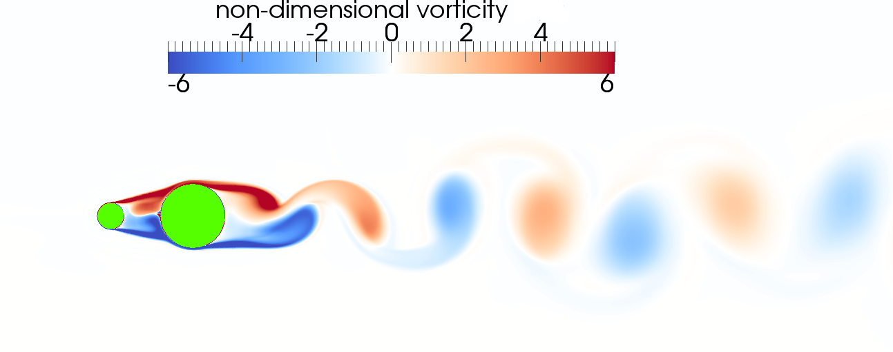
Figure 2: An instanteous plot showing contours of vorticity in the wake behind the cylinder pair from figure 1.
After analysing the results, the CFD engineer can perform additional simulations. These cases can optimise the design by altering angles or wind speeds, or evaluating the effects of changing the geometry.
For examples of how CFD can help you, see our sector pages.
References:
[1] Anderson, J. D. “Fundamentals of aerodynamics“ 3rd edition, MacGraw-Hill, 2001.
[3] Wilcox, David C. “Turbulence modeling for CFD“ 2nd edition, DCW industries, 1998.